PCA in itself uses projection, which is a linear method. Because of it, the performance on non-linear data is not optimal. That’s where Kernel PCA comes in.
What is it?
Kernel PCA, or kPCA, is an extension of the traditional PCA method for Dimensionality Reduction most commonly used in Machine Learning.
As the name suggests, it uses the Kernel Trick, which identifies linear high-dimensional relations that become complex non-linear projections when the dimension is reduced.
This works much better than the traditional PCA for non-linear data. Kernel PCA also can cluster instances better than PCA for non-linear data.
Kernel PCA can cluster and linearly separate non-linear data, even if it doesn’t reduce dimensionality.
How does it work?
The main difference between Kernel PCA and PCA is that kPCA doesn’t compute the principal components itself, but rather the projection of data into these components from a higher dimensionality.
Using a given kernel function it implicitly maps data into a higher-dimension feature space, where the data is linearly separable, and then it projects the data back to the desirable dimensionality.
Some common kernel functions are:
-
Linear
Which would be the same as traditional PCA.
-
Polynomial
More flexible than linear, but data needs to follow the shape of the function.
-
Sigmoid
Follows the Sigmoid Function, used in Logistic Regression.
-
Radial Basis Function (RBF)
Also known as the Gaussian kernel, maps normal curves around all data.
-
Cosine
Measures the cosine of the angle between vectors. Better used when similarity depends on direction rather than magnitude.
Using scikit-learn
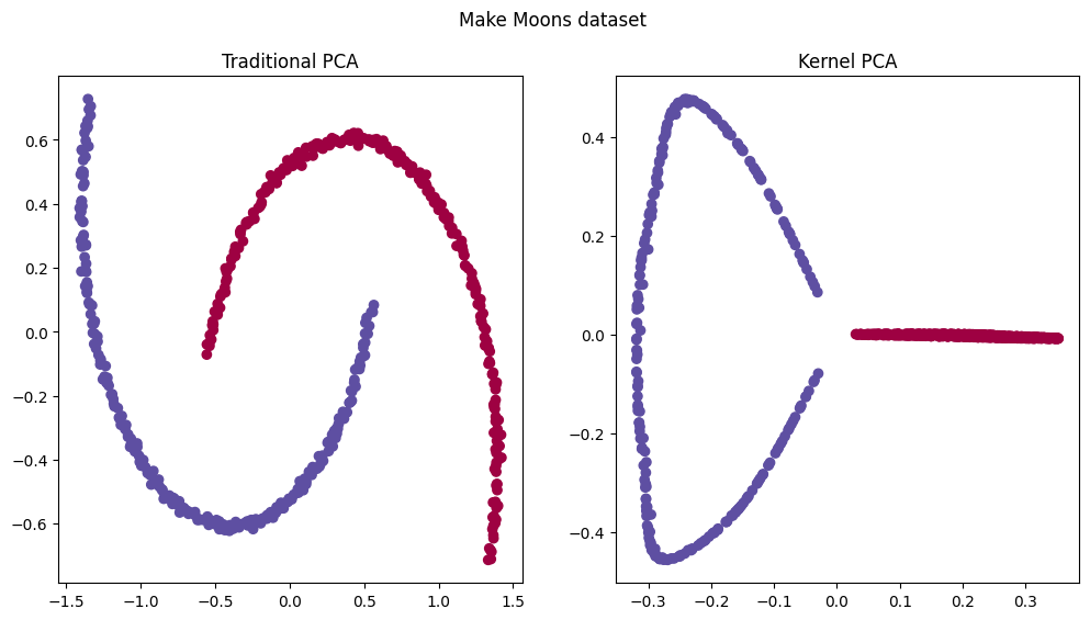
In practice, kPCA uses the same trick as using Nystroem approximation in linear regression to adapt to non-liner data. We can fit linear algorithms to non-linear data if applying kPCA before the estimator.
For example, given the make moons dataset, would be impossible to fit a linear classification algorithm, but using kPCA the algorithm can draw a linear decision boundary in higher-dimensionality as seen from the image above. That translates to a non-linear classification, as seen below.
from sklearn.pipeline import make_pipeline
from sklearn.decomposition import KernelPCA
from sklearn.linear_model import LogisticRegression
from sklearn.inspection import DecisionBoundaryDisplay
import matplotlib.pyplot as plt

pipeline = make_pipeline(KernelPCA(kernel="rbf"), LogisticRegression(C=10e5))
X_train, X_test, y_train, y_test = train_test_split(X, y)

pipeline.fit(X_train, y_train)

plot = DecisionBoundaryDisplay.from_estimator(
	pipeline, X_test, response_method="predict",
	alpha=0.2,cmap=plt.cm.Spectral
)

plot.ax_.scatter(X[:, 0], X[:, 1], c=y, cmap=plt.cm.Spectral)